
Revit project geolocation and data scraping
Automating project start-up in Revit. Geolocation, point clouds, site data imports and more.
Introduction
In this post I want to show you the kinds of data you may come across, how they can be processed, and how they can be used in the design and analysis of buildings and structures. At the end I will outline how all of this can be automated in Revit and Blender.
Public data has become more and more accessible lately. Government institutions, as well as amateur data collection and analysis, give us access to amazing resources. All it takes is to process them, and we can create design conditions unprecedented in our industry, without much extra work.
I remember when sun analysis was done with a special ruler laid over the floor plan: a standardised practice with an enormous number of simplifications. Then we moved on to 3D sun studies, building our design in three dimensions and modelling simple masses of the neighbouring buildings. We did not necessarily check whether our software took UTC offsets into account, whether it considered elevation above sea level, whether it assumed a flat plane or the curvature of the Earth… but that may be a topic for another post.
The example above is meant to show the possibilities in front of us and how deep we can go with analysis. Of course, more complex analyses take time to enter or model the necessary data.
DTM – a digital terrain model, but is it really?
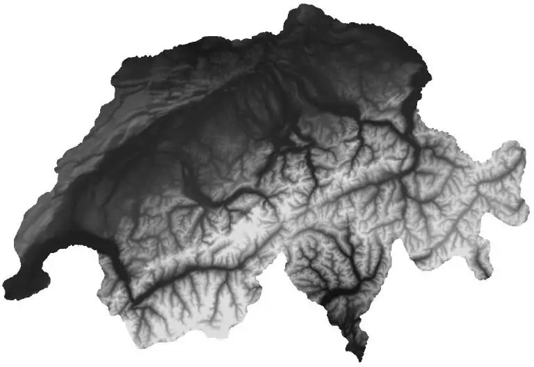
We have reached the point where most geographic data is publicly available on the internet. It started with DEMs (digital elevation models): satellite imagery describing terrain height. When I first became interested, the scales were rather coarse, since one pixel covered about 30 × 30 m of terrain. Later it went down to 10 × 10 m. From such data you could already extract quite an interesting simplification of the terrain, at no extra cost.
Examples:
- ALOS World 3D - 30 m
- NASADEM Global Digital Elevation Model
- USGS 1/3 arc-second Digital Elevation Model - 10 m resolution
At some point databases appeared where you could query the elevation above sea level, such as:
- https://www.opentopography.org/
- https://open-elevation.com/
- or even the Google Maps API with elevation data.
Today you can find DEMs with a resolution of 1 m. A good example are the elevation packages published by Poland, covering the whole country with points spaced every 1 m. DEMs come in a couple of kinds:
- raster
- grid
The first is, for example, a .tiff image in which the shade of grey defines the height. The limit here is the size of one pixel (e.g. 30 m, 10 m, 1 m). Processing such data calls for free software such as QGIS. QGIS can load such a tiff in the right coordinates, clip it to the extent we need and then generate, for example, contour lines or a point grid from the raster. A grid is, for example, a text file with a list of numbers defining the height above sea level on a 1 m grid. To use it in Revit, for example, you need to convert the data to a CSV file with X, Y and Z columns. That lets you import it as a toposurface.
But is this really the limit of detail? Of course not. 😉
Point clouds
The next level of detail, in my view, is raw survey data. In the past this meant crowds of surveyors and advanced triangulation technology. Today it is still based on triangulation, only the amount of data has grown exponentially. I am talking about point clouds. Here we can check accuracy with a margin of error of a few centimetres or, for airborne lidar, taking the Polish geoportal as an example, a density from 4 points/m² up to 20 points/m² in larger cities, with a mean height error of around 10 cm.
Again I will use the example of the Polish ministry, which publishes survey data (lidar) in the LAS format. A point cloud is something like an image in three dimensions. Instead of pixels we have points in 3D. Each point can carry additional attributes, such as:
- colour
- classification – is it a building, low vegetation, high vegetation, ground, a car, a street lamp…
- accuracy – how precise the measurement of the point was
- intensity – the intensity of the reflected lidar beam
- and plenty of other direct data
- plus indirect data from analysing points and their relations, e.g.:
- are the points on one plane – could it be a wall?
- do the points form a group without any plane – could it be a tree?
That is a huge amount of data to work with. The Polish geoportal calls it survey data; I will use the general term, point cloud. Point clouds can be divided in all sorts of ways; I will focus on a practical split:
- lidar point clouds
- photogrammetry point clouds
and another one:
- classified point clouds
- unclassified point clouds
Finally, clouds can also be:
- registered,
- unregistered.
If you hear the term, it mostly means placing the cloud in specific horizontal and vertical coordinate systems and cleaning it of gaps and erroneous measurements. In short: geolocation.
The Polish geoportal usually provides fully merged survey data with the basic information we need:
- geolocation
- colour
- classification
Thanks to this we can quickly and easily refine such a cloud for design purposes:
- Filter all buildings onto a separate layer, to measure the neighbours.
- Filter the ground and generate 3D terrain from it (e.g. a Revit toposurface).
- Filter high vegetation, process the data and find the tree tops (and therefore the tree locations).
- With free tools, filter all points within our plot boundary and remove everything but the ground points, leaving the rest of the cloud untouched.
The perfect tool for these tasks is CloudCompare. It opens point clouds while keeping their reference system, and it can clean, analyse and process the data. It also has basic point classification. Of its strengths, the ones I find most useful in the design process are:
- classifying ground points (if there is no classification)
- projecting colours from satellite images onto the point cloud (if colours are missing)
- registering point clouds against each other
These steps let us split the point cloud into light packages that can then be linked into a Revit file, with full control over visibility. Unfortunately you cannot avoid the paid Autodesk ReCap here: it opens .las files and saves them as .rcp, which Revit can load.
With the cloud prepared this way we can load it into our project in the right coordinates and be sure the points sit exactly on the terrain. From experience I can say such a cloud works great at the concept stage and for designing in the context of real (!!!) site features: vegetation, watercourses, buildings, roads, slopes, sculptures (no point listing them, it is literally everything). It helps to detail and model the roofs of neighbouring buildings, or to check the actual heights of parapets and buildings. It also works great for visualisation, for generating the real terrain and for analysing earthworks.
Plot boundaries
Different countries have different public databases. Examples of such services:
- WMS (Web Map Service), WMTS (Web Map Tile Service),
- WFS (Web Feature Service),
- ATOM,
- INSPIRE (Infrastructure for Spatial Information in Europe).
These are standardised services for sharing geographic data such as orthophoto maps, boundaries, local zoning plans and much more.
The Polish geoportal lets you download the BDOT10k database (topographic objects database), from which, using our familiar QGIS, we can extract plot boundaries, outlines of existing buildings, road centrelines and much more, such as bus stop locations, land use types etc. Such data can then be imported into 2D or 3D design software.
QGIS lets us filter it visually and place it in the right coordinates: so-called reprojection from the national coordinate system to the one the project is drawn in. More on that in the next section. This link shows which WMS services geoportal.gov.pl offers.
Geolocation and EPSG codes
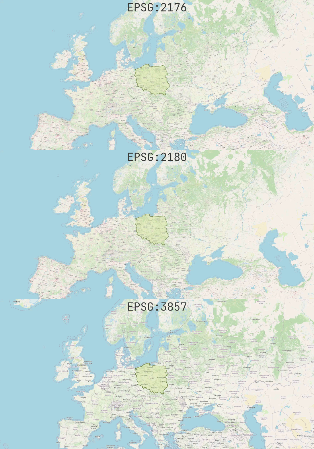 This is where we should have started, but it is always better to start with something more spectacular. EPSG, however, is the piece of the puzzle that ties everything together. Knowing it makes the work easier, eliminates basic mistakes and, with almost no effort, introduces the first process automation.
EPSG codes were created to standardise the names of coordinate systems. They cover both projected (planar) and geographic coordinate systems.
In Poland we have two reference frames: the older PL-ETRF89 and the current PL-ETRF2000.
The Polish planar coordinate systems with their EPSG codes are:
| EPSG | System | Central meridian |
|---|---|---|
| EPSG:2180 | PL-1992 | 19° (whole country) |
| EPSG:2176 | PL-2000 zone 5 | 15° |
| EPSG:2177 | PL-2000 zone 6 | 18° |
| EPSG:2178 | PL-2000 zone 7 | 21° |
| EPSG:2179 | PL-2000 zone 8 | 24° |
Knowing which system the plot, or our data, is in lets us merge the data without trouble. QGIS is again the best tool for analysing and processing it. It often happens that the point cloud comes in the national system while the project is set up in local coordinates, e.g. zone 6.
Building models
For buildings we have a few options for generating 3D models. The first, easier but time-consuming option is to find existing models and place them in 3D on the building footprints obtained from WFS services. It is an obvious option, but worth mentioning, because sometimes you come across very accurate models.
The second option is to get the data from the geoportal. Buildings can be downloaded as GML at LOD1. To use them in Revit or another program, they have to be converted to a native format: for Revit preferably a MASS FAMILY, for Blender e.g. OBJ. A GML file has an XML structure, so we can read it in Python with an XML parser. It would look like this:
# python
import numpy as np
from xml.etree import ElementTree as et

FILEPATH = "file.gml"


def unflatten(coords, s=1):
    """gets numbers list
    returns array of points (XYZ)"""
    verts = np.array([(coords[i] * s, coords[i + 1] * s, coords[i + 2] * s) for i in range(0, len(coords), 3)])
    return verts


tree = et.parse(FILEPATH)
polygons = tree.findall(".//{http://www.opengis.net/gml}Polygon")
verts = []
faces = []
for i, p in enumerate(polygons):
    poslist = p.find(".//{http://www.opengis.net/gml}posList")
    text = poslist.text
    coords = [float(i) for i in text.split(" ")]
    points = unflatten(coords)
    start_idx = len(verts)
    end_idx = start_idx + len(points)

    verts.extend(points)
    faces.append([i for i in range(start_idx, end_idx)])
This gives us a set of vertices and polygons (groups of vertices forming single polygons). From this format it is very easy to generate an object in Blender, save it as OBJ and import it into Revit. Or, with the Revit API, to model MASS objects from this data automatically. The advantage of this solution is that the buildings are already located horizontally and vertically.
The large-distance problem
There is one problem well known among 3D artists. The further a vertex is from the point [0,0,0], the more “approximate” its display becomes. It comes from how computers handle decimal numbers. A computer always approximates decimals in its own representation, so it can happen that when comparing 0.003 == 0.003, the numbers turn out different, because to the computer 0.003 = 0.003000000000000001. The solution would be to read the location of the
internal originorproject base pointand move all vertices by that vector, so they are placed relative to a nearby insertion point rather than through shared coordinates.
The last solution I would suggest requires a bit more technical knowledge, but it is the most accurate: generating the building geometry from the point cloud. Plenty of spatial analysis algorithms come to help here, but in short we can split it into the following tasks:
- extract the points classified as buildings from the point cloud,
- analyse which points belong to which planes and group them by plane,
- with planes and their points, find the boundary points (lying on the edges of each group); this gives approximate edges of the object and its planes,
- remove points that lie on one straight line or within a small distance of it; what remains are the vertices,
- merge vertices that lie close to each other, number them and assign them to planes,
- the final result gives the same sets of vertices and polygons as the script above.
This option gives much more detailed buildings. If we need more detail, we can use lidar, a drone, a camera or a smartphone to generate additional point clouds, for example with the free Meshroom (photogrammetry turns photos from cameras and smartphones into point clouds). We can then merge our point cloud with the one from the geoportal, densifying it and filling the gaps. Aligning a cloud without coordinates with a cloud that has them is called registration. It also involves cleaning the cloud of erroneous measurements.
Satellite images
Would you believe me if I told you there is an image format that stores the image’s location in coordinates? Imagine you get a local zoning plan, a scanned map from the investor, a satellite image of the plot or any other map. You drop it into your software and it always lands exactly in the right place? Exactly to scale? Without any distortion?
Yes, it is possible. Not always and not in every program, but geolocation can be stored for an image, for example in PDF or TIFF files. Such TIFF files are called GeoTIFF.
When you download a satellite image from a government portal, it usually already has its coordinates and coordinate system set. Drop such a TIFF into QGIS, set the system it was saved in (e.g. EPSG:2180), and it lands right in place. No distortion, no shift. Perfect.
The second strength of satellite images is the data. Colour may be useful to us: for a point cloud without colour data, we can project the colours of a satellite image onto it. CloudCompare can do that, for example.
Joining it together and automating
The most interesting part of the puzzle is that most of these tasks can be reduced to a single button, e.g. in Revit. We only need to enter a few parameters:
- location (coordinates)
- radius (how far around to fetch data)
- optionally a polygon/region with the plot boundary
The script does the rest: it fetches the terrain, point cloud, plot boundaries, buildings and orthophoto map and places them in the right coordinate system. The designer gets a ready site context in minutes instead of days.